
Initiate by creating an account on the official Spotify website, which is completely free and requires very little work.
Then, go to your application dashboard and choose “Create an app.” Fill in the blanks and get ready to explore.
Start your favorite Python IDE using your ClientID and Client Secret. It’s time to start coding.
Instead of hitting the endpoints directly, we’ll utilize SpotiPy, a wrapper over the Spotify API, to perform attractive one-line calls. Let’s get things set up.
!pip install spotipy
The spotipy is then initialized. The Spotify developer’s passwords are kept in the variables CLIENT_ID and CLIENT_SECRET of the Spotify object.
import spotipy
	from spotipy.oauth2 import SpotifyClientCredentials
	client_credentials_manager = SpotifyClientCredentials(client_id=CLIENT_ID, client_secret=CLIENT_SECRET)
	sp = spotipy.Spotify(client_credentials_manager=client_credentials_manager)
Scrape Artists and Tracks
Data querying is the next stage. Note that you can only get information on 50 tracks at a time. You may search for specific objects using the q argument in the sp.search() function.
artist_name = []
	track_name = []
	track_popularity = []
	artist_id = []
	track_id = []
	for i in range(0,1000,50):
	    track_results = sp.search(q='year:2021', type='track', limit=50,offset=i)
	    for i, t in enumerate(track_results['tracks']['items']):
	        artist_name.append(t['artists'][0]['name'])
	        artist_id.append(t['artists'][0]['id'])
	        track_name.append(t['name'])
	        track_id.append(t['id'])
	        track_popularity.append(t['popularity'])
Place the queried information into the Pandas Dataframe
import pandas as pd
track_df = pd.DataFrame({'artist_name' : artist_name, 'track_name' : track_name, 'track_id' : track_id, 'track_popularity' : track_popularity, 'artist_id' : artist_id})
print(track_df.shape)
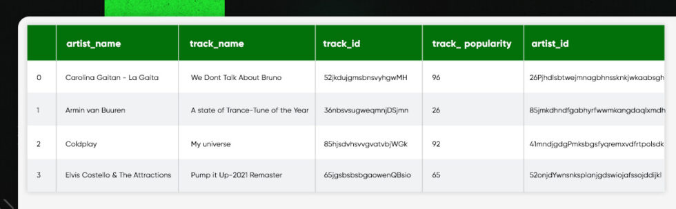
track_df.head()
artist_popularity = []
	artist_genres = []
	artist_followers = []
	for a_id in track_df.artist_id:
	  artist = sp.artist(a_id)
	  artist_popularity.append(artist['popularity'])
	  artist_genres.append(artist['genres'])
	  artist_followers.append(artist['followers']['total'])
Add the track_df data frame
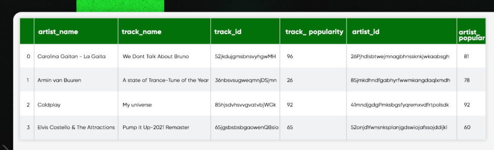
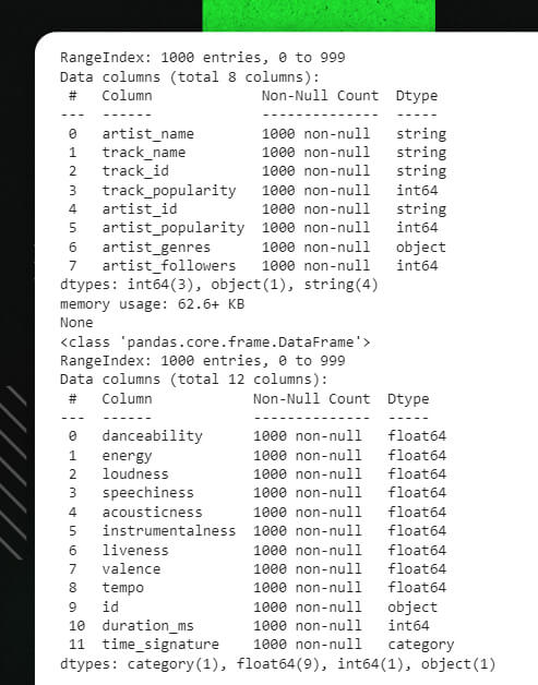
track_df = track_df.assign(artist_popularity=artist_popularity, artist_genres=artist_genres, artist_followers=artist_followers)
	track_df.head()
Numerical Features of Retrieval Tracks
You will then plunge into numerical analysis of music, but first, you will need to gather some information. Fortunately, Spotify will offer you with detailed information on 82 million songs, which is ideal for our needs.
To begin, go to the Spotify API reference page to learn about the features that contribute to a track’s profile.
Second, get the characteristics of the tracks and put them in the data frame.
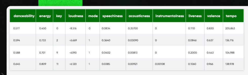
track_features = []
	for t_id in track_df['track_id']:
	  af = sp.audio_features(t_id)
	  track_features.append(af)
	tf_df = pd.DataFrame(columns = ['danceability', 'energy', 'key', 'loudness', 'mode', 'speechiness', 'acousticness', 'instrumentalness', 'liveness', 'valence', 'tempo', 'type', 'id', 'uri', 'track_href', 'analysis_url', 'duration_ms', 'time_signature'])
	for item in track_features:
	  for feat in item:
	    tf_df = tf_df.append(feat, ignore_index=True)
	tf_df.head()
The features data frame for the songs looks like this:
Let’s remove some few unnecessary columns and examine the data frames’ structure:
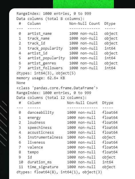
cols_to_drop2 = ['key','mode','type', 'uri','track_href','analysis_url']
	tf_df = tf_df.drop(columns=cols_to_drop2)
	print(track_df.info())
	print(tf_df.info())
Reading the data into a data frame using Pandas
Column types inference is the last step before data exploration and visualization.
track_df['artist_name'] = track_df['artist_name'].astype("string")
	track_df['track_name'] = track_df['track_name'].astype("string")
	track_df['track_id'] = track_df['track_id'].astype("string")
	track_df['artist_id'] = track_df['artist_id'].astype("string")
	tf_df['duration_ms'] = pd.to_numeric(tf_df['duration_ms'])
	tf_df['instrumentalness'] = pd.to_numeric(tf_df['instrumentalness'])
	tf_df['time_signature'] = tf_df['time_signature'].astype("category")
	print(track_df.info())
	print(tf_df.info())
The data frames that result have the following structure:
Exploring 2021 Trends
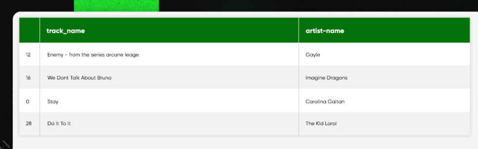
Are you in search of popular tracks of 2021?
track_df.sort_values(by=['track_popularity'], ascending=False)[['track_name', 'artist_name']].head(20)
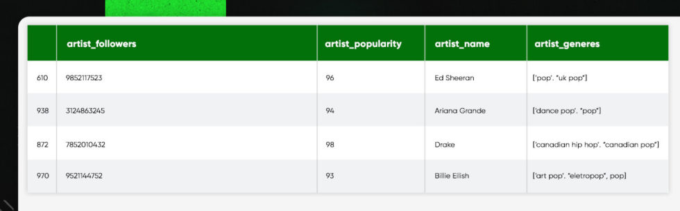
Who is Most Followed?
by_art_fol = pd.DataFrame(track_df.sort_values(by=['artist_followers'], ascending=False)[['artist_followers','artist_popularity', 'artist_name','artist_genres']])
	by_art_fol.astype(str).drop_duplicates().head(20)
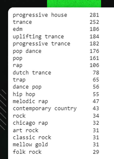
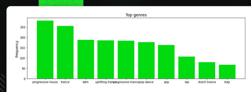
Let’s examine how many genres the track_df data frame contains:
def to_1D(series):
	 return pd.Series([x for _list in series for x in _list])
	to_1D(track_df['artist_genres']).value_counts().head(20)
Visualizing the above results:
import matplotlib.pyplot as plt
	fig, ax = plt.subplots(figsize = (14,4))
	ax.bar(to_1D(track_df['artist_genres']).value_counts().index[:10],
	        to_1D(track_df['artist_genres']).value_counts().values[:10])
	ax.set_ylabel("Frequency", size = 12)
	ax.set_title("Top genres", size = 14)
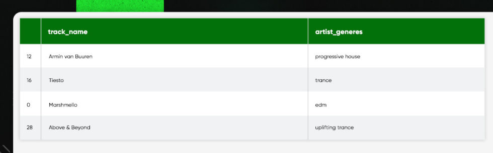
Searching for the top 10 artists filtered by the number of the followers
top_10_genres = list(to_1D(track_df['artist_genres']).value_counts().index[:20])
	top_artists_by_genre = []
	for genre in top_10_genres:
	  for index, row in by_art_fol.iterrows():
	    if genre in row['artist_genres']:
	      top_artists_by_genre.append({'artist_name':row['artist_name'], 'artist_genre':genre})
	      break
	pd.json_normalize(top_artists_by_genre)
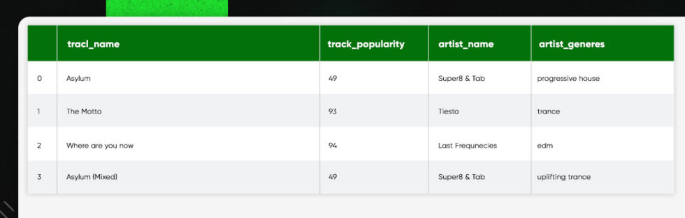
Searching for the top 20 filtered by popularity for every top 10 genres:
by_track_pop = pd.DataFrame(track_df.sort_values(by=['track_popularity'], ascending=False)[['track_popularity','track_name', 'artist_name','artist_genres', 'track_id']])
	by_track_pop.astype(str).drop_duplicates().head(20)
	top_songs_by_genre = []
	for genre in top_10_genres:
	  for index, row in by_track_pop.iterrows():
	    if genre in row['artist_genres']:
	      top_songs_by_genre.append({'track_name':row['track_name'], 'track_popularity':row['track_popularity'],'artist_name':row['artist_name'], 'artist_genre':genre})
	      break
	pd.json_normalize(top_songs_by_genre)
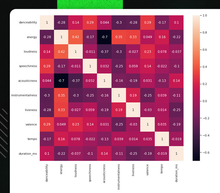
Visualizing Features of the Tracks
import seaborn as sn
	sn.set(rc = {'figure.figsize':(12,10)})
	sn.heatmap(tf_df.corr(), annot=True)
	plt.show()
A multivariate KDE might also be plotted for a specific pair of variables:
sn.set(rc = {'figure.figsize':(20,20)})
	sn.jointplot(data=tf_df, x="loudness", y="energy", kind="kde")

What distinguishes the most popular tracks from the rest of the dataset? Here, we will learn by producing a feature portrait of the relevant sets based on the mean values of selected characteristics.
feat_cols = ['danceability', 'energy', 'speechiness', 'acousticness', 'instrumentalness', 'liveness', 'valence']
	top_100_feat = pd.DataFrame(columns=feat_cols)
	for i, track in by_track_pop[:100].iterrows():
	  features = tf_df[tf_df['id'] == track['track_id']]
	  top_100_feat = top_100_feat.append(features, ignore_index=True)
	top_100_feat = top_100_feat[feat_cols]


	from sklearn import preprocessing
	mean_vals = pd.DataFrame(columns=feat_cols)
	mean_vals = mean_vals.append(top_100_feat.mean(), ignore_index=True)
	mean_vals = mean_vals.append(tf_df[feat_cols].mean(), ignore_index=True)
	print(mean_vals)


	import plotly.graph_objects as go
	import plotly.offline as pyo
	fig = go.Figure(
	    data=[
	        go.Scatterpolar(r=mean_vals.iloc[0], theta=feat_cols, fill='toself', name='Top 100'),
	        go.Scatterpolar(r=mean_vals.iloc[1], theta=feat_cols, fill='toself', name='All'),
	    ],
	    layout=go.Layout(
	        title=go.layout.Title(text='Feature comparison'),
	        polar={'radialaxis': {'visible': True}},
	        showlegend=True
	    )
	)


	#pyo.plot(fig)
	fig.show()
The most famous songs appear to be slightly more rhythmic and have more positivity. They’re also devoid of efficiency, effectiveness and vibrancy.
Get Suggestions
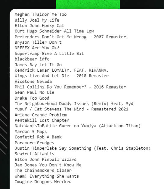
Our research concludes with music recommendations based on artist_id, genre, and track id. Spotify never runs out of content recommendations since the output is randomized.
rec = sp.recommendations(seed_artists=["3PhoLpVuITZKcymswpck5b"], seed_genres=["pop"], seed_tracks=["1r9xUipOqoNwggBpENDsvJ"], limit=100)
	for track in rec['tracks']:
	  print(track['artists'][0]['name'], track['name'])
This blog will help you understand the idea regarding Spotify Web APIs methods and how the fetched information will be visualized and analyzed.
For any web scraping services, contact X-Byte Enterprise Crawling today!
Request for a quote!
 ✯ Alpesh Khunt ✯