Whether you believe it or not, but guest reviews affect people’s bookings and travel.
What does your experience say? It is obvious that when you are looking for a vacation on Expedia, Tripadvisor, or Booking.com, what would be your action?
You will surely check on the reviews before you confirm. If you are still confused regarding how guest reviews are important, then you can check the below image:
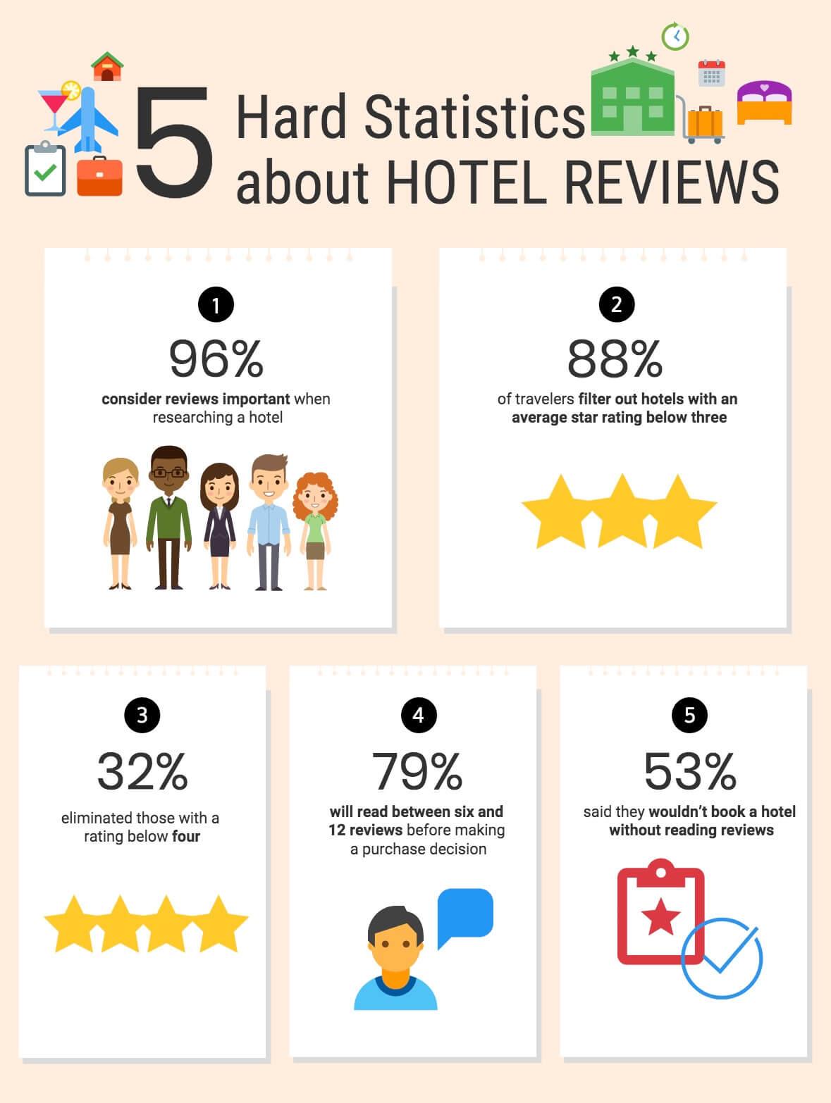
Guest reviews impact people’s decisions, which means it is preferable to consider what people are saying about the hotel. Not only do you read the reviews, but also observe in a manner that you learn the most. The reviews will brief if you are fulfilling your customer’s expectations. This is vital for developing marketing policies depending on the personas of customers.
What is Sentiment Analysis?
Sentiment analysis, also known as opinion mining, is a review extraction of hotel data, whether positive, negative, or neutral and will provide a sentiment score. This method is technically used on reviews or social media.
In this blog, we will highlight how to efficiently fetch restaurant reviews using a web scraping tool and undergo web scraping using Python.
The Python code is found here.
Load the libraries
library(dplyr)
library(readr)
library(lubridate)
library(ggplot2)
library(tidytext)
library(tidyverse)
library(stringr)
library(tidyr)
library(scales)
library(broom)
library(purrr)
library(widyr)
library(igraph)
library(ggraph)
library(SnowballC)
library(wordcloud)
library(reshape2)
theme_set(theme_minimal())
The Data
df <- read_csv("Hilton_Hawaiian_Village_Waikiki_Beach_Resort-Honolulu_Oahu_Hawaii__en.csv")
df <- df[complete.cases(df), ]
df$review_date <- as.Date(df$review_date, format = "%d-%B-%y")dim(df); min(df$review_date); max(df$review_date)
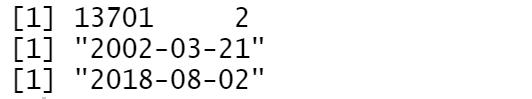
As per the records of Hilton Hawaiian from TripAdvisor, there are 13,701 English reviews from the dates 2002-03-21 to 2018-08-02.
df %>%
count(Week = round_date(review_date, "week")) %>%
ggplot(aes(Week, n)) +
geom_line() +
ggtitle('The Number of Reviews Per Week')
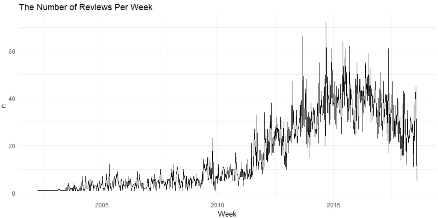 The maximum number of weekly reviews were received at the end of 2014. The hotel received over 70 appraisals that week.
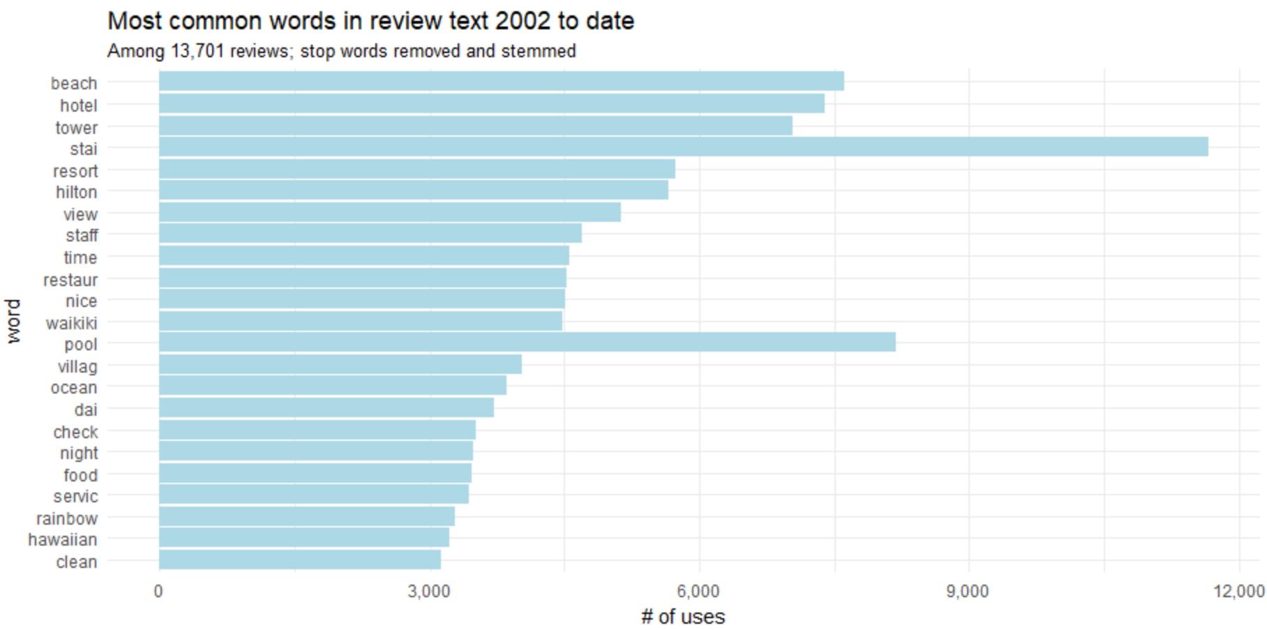
  df <- tibble::rowid_to_column(df, "ID")
  df <- df %>%
  mutate(review_date = as.POSIXct(review_date, origin = "1970-01-01"),month = round_date(review_date, "month"))review_words <- df %>%
  distinct(review_body, .keep_all = TRUE) %>%
  unnest_tokens(word, review_body, drop = FALSE) %>%
  distinct(ID, word, .keep_all = TRUE) %>%
  anti_join(stop_words, by = "word") %>%
  filter(str_detect(word, "[^\\d]")) %>%
  group_by(word) %>%
  mutate(word_total = n()) %>%
  ungroup()word_counts <- review_words %>%
  count(word, sort = TRUE)word_counts %>%
  head(25) %>%
  mutate(word = reorder(word, n)) %>%
  ggplot(aes(word, n)) +
  geom_col(fill = "lightblue") +
  scale_y_continuous(labels = comma_format()) +
  coord_flip() +
  labs(title = "Most common words in review text 2002 to date",
  subtitle = "Among 13,701 reviews; stop words removed",
  y = "# of uses")
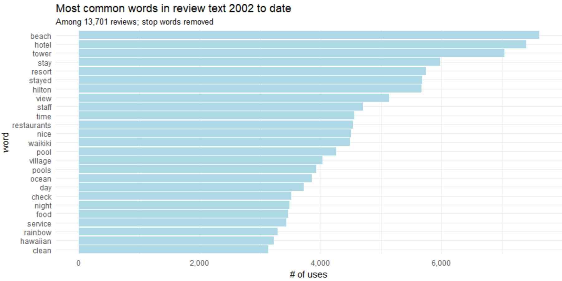
We can ofcourse merge “stay” and “stayed” and “pool” and “pools”. Stemming is the process of decreasing inflected arguments to their word stem, base or root format.
word_counts %>%
head(25) %>%
mutate(word = wordStem(word)) %>%
mutate(word = reorder(word, n)) %>%
ggplot(aes(word, n)) +
geom_col(fill = "lightblue") +
scale_y_continuous(labels = comma_format()) +
coord_flip() +
labs(title = "Most common words in review text 2002 to date",
subtitle = "Among 13,701 reviews; stop words removed and stemmed",
y = "# of uses")
Role of Web Scraping
Bigrams
We frequently try to learn the relationship between the words in an analysis. What should be the categorization of words across the analysis text? From the given sentences, which word is most likely to follow? Which words are strongly connected? Hence, several exciting text type of research is based on the relationships.
“Bigrams”, are defined when we examine a pair of two consecutive words.
So, here is the code to display the reviews of Hilton Hawaiian’s village’s from TripAdvisor.
  review_bigrams <- df %>%
  unnest_tokens(bigram, review_body, token = "ngrams", n = 2)bigrams_separated <- review_bigrams %>%
  separate(bigram, c("word1", "word2"), sep = " ")bigrams_filtered <- bigrams_separated %>%
  filter(!word1 %in% stop_words$word) %>%
  filter(!word2 %in% stop_words$word)bigram_counts <- bigrams_filtered %>%
  count(word1, word2, sort = TRUE)bigrams_united <- bigrams_filtered %>%
  unite(bigram, word1, word2, sep = " ")bigrams_united %>%
  count(bigram, sort = TRUE)
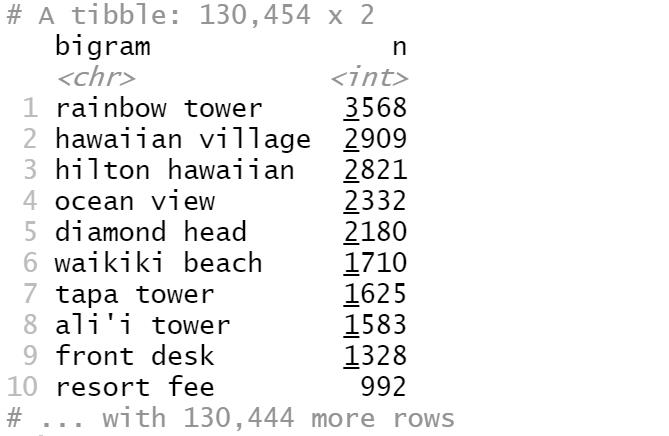
The most common bigrams is “rainbow tower”, followed by “Hawaiian village”.
One writes the script of bigrams in word network as below:
review_subject <- df %>%
  unnest_tokens(word, review_body) %>%
  anti_join(stop_words)my_stopwords <- data_frame(word = c(as.character(1:10)))
  review_subject <- review_subject %>%
  anti_join(my_stopwords)title_word_pairs <- review_subject %>%
  pairwise_count(word, ID, sort = TRUE, upper = FALSE)set.seed(1234)
  title_word_pairs %>%
  filter(n >= 1000) %>%
  graph_from_data_frame() %>%
  ggraph(layout = "fr") +
  geom_edge_link(aes(edge_alpha = n, edge_width = n), edge_colour = "cyan4") +
  geom_node_point(size = 5) +
  geom_node_text(aes(label = name), repel = TRUE,
                 point.padding = unit(0.2, "lines")) +
  ggtitle('Word network in TripAdvisor reviews')
  theme_void()
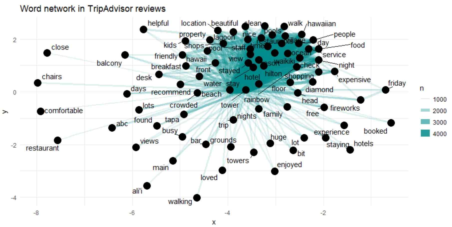
The above picture shows the common bigrams in TripAdvisor reviews, showing those that took place almost 1000 times and neither word was a stop-word.
The above graph shows association between the top numerous words (“Hawaiian”, “village”, “ocean”, and “view”).
However, we could not see the strong cluster structure in the network.
Trigrams
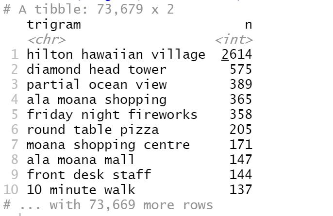
Let us check the common trigrams for Hilton Hawaiian Village’s reviews.
review_trigrams <- df %>%
  unnest_tokens(trigram, review_body, token = "ngrams", n = 3)

trigrams_separated <- review_trigrams %>%
  separate(trigram, c("word1", "word2", "word3"), sep = " ")

trigrams_filtered <- trigrams_separated %>%
  filter(!word1 %in% stop_words$word) %>%
  filter(!word2 %in% stop_words$word) %>%
  filter(!word3 %in% stop_words$word)

trigram_counts <- trigrams_filtered %>%
  count(word1, word2, word3, sort = TRUE)

trigrams_united <- trigrams_filtered %>%
  unite(trigram, word1, word2, word3, sep = " ")

trigrams_united %>%
  count(trigram, sort = TRUE)
  review_trigrams <- df %>%
  unnest_tokens(trigram, review_body, token = "ngrams", n = 3)

trigrams_separated <- review_trigrams %>%
  separate(trigram, c("word1", "word2", "word3"), sep = " ")

trigrams_filtered <- trigrams_separated %>%
  filter(!word1 %in% stop_words$word) %>%
  filter(!word2 %in% stop_words$word) %>%
  filter(!word3 %in% stop_words$word)

trigram_counts <- trigrams_filtered %>%
  count(word1, word2, word3, sort = TRUE)

trigrams_united <- trigrams_filtered %>%
  unite(trigram, word1, word2, word3, sep = " ")

trigrams_united %>%
  count(trigram, sort = TRUE)
Important Words Highlighted In Reviews
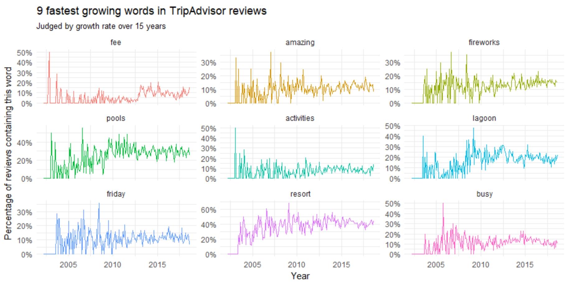
Which kind of words or topics has become more consistent, or less consistent, over the period? These results in providing an idea of the hotel’s changing ecosystem, for instance, service, renovation, issue-resolving, and prediction of topics that will continue to rise in 2003 significance.
  reviews_per_month <- df %>%
  group_by(month) %>%
  summarize(month_total = n())word_month_counts <- review_words %>%
  filter(word_total >= 1000) %>%
  count(word, month) %>%
  complete(word, month, fill = list(n = 0)) %>%
  inner_join(reviews_per_month, by = "month") %>%
  mutate(percent = n / month_total) %>%
  mutate(year = year(month) + yday(month) / 365)mod <- ~ glm(cbind(n, month_total - n) ~ year, ., family = "binomial")slopes <- word_month_counts %>%
  nest(-word) %>%
  mutate(model = map(data, mod)) %>%
  unnest(map(model, tidy)) %>%
  filter(term == "year") %>%
  arrange(desc(estimate))slopes %>%
  head(9) %>%
  inner_join(word_month_counts, by = "word") %>%
  mutate(word = reorder(word, -estimate)) %>%
  ggplot(aes(month, n / month_total, color = word)) +
  geom_line(show.legend = FALSE) +
  scale_y_continuous(labels = percent_format()) +
  facet_wrap(~ word, scales = "free_y") +
  expand_limits(y = 0) +
  labs(x = "Year",
       y = "Percentage of reviews containing this word",
       title = "9 fastest growing words in TripAdvisor reviews",
       subtitle = "Judged by growth rate over 15 years")
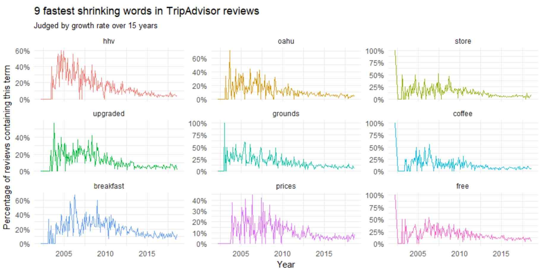
Let us find the words using Python script that decreases the words frequency in review.
slopes %>%
tail(9) %>%
inner_join(word_month_counts, by = "word") %>%
mutate(word = reorder(word, estimate)) %>%
ggplot(aes(month, n / month_total, color = word)) +
geom_line(show.legend = FALSE) +
scale_y_continuous(labels = percent_format()) +
facet_wrap(~ word, scales = "free_y") +
expand_limits(y = 0) +
labs(x = "Year",
y = "Percentage of reviews containing this term",
title = "9 fastest shrinking words in TripAdvisor reviews",
subtitle = "Judged by growth rate over 4 years")
Now, let us compare few words of TripAdvisor reviews using Python script
word_month_counts %>%
filter(word %in% c("service", "food")) %>%
ggplot(aes(month, n / month_total, color = word)) +
geom_line(size = 1, alpha = .8) +
scale_y_continuous(labels = percent_format()) +
expand_limits(y = 0) +
labs(x = "Year",
y = "Percentage of reviews containing this term", title = "service vs food in terms of reviewers interest")
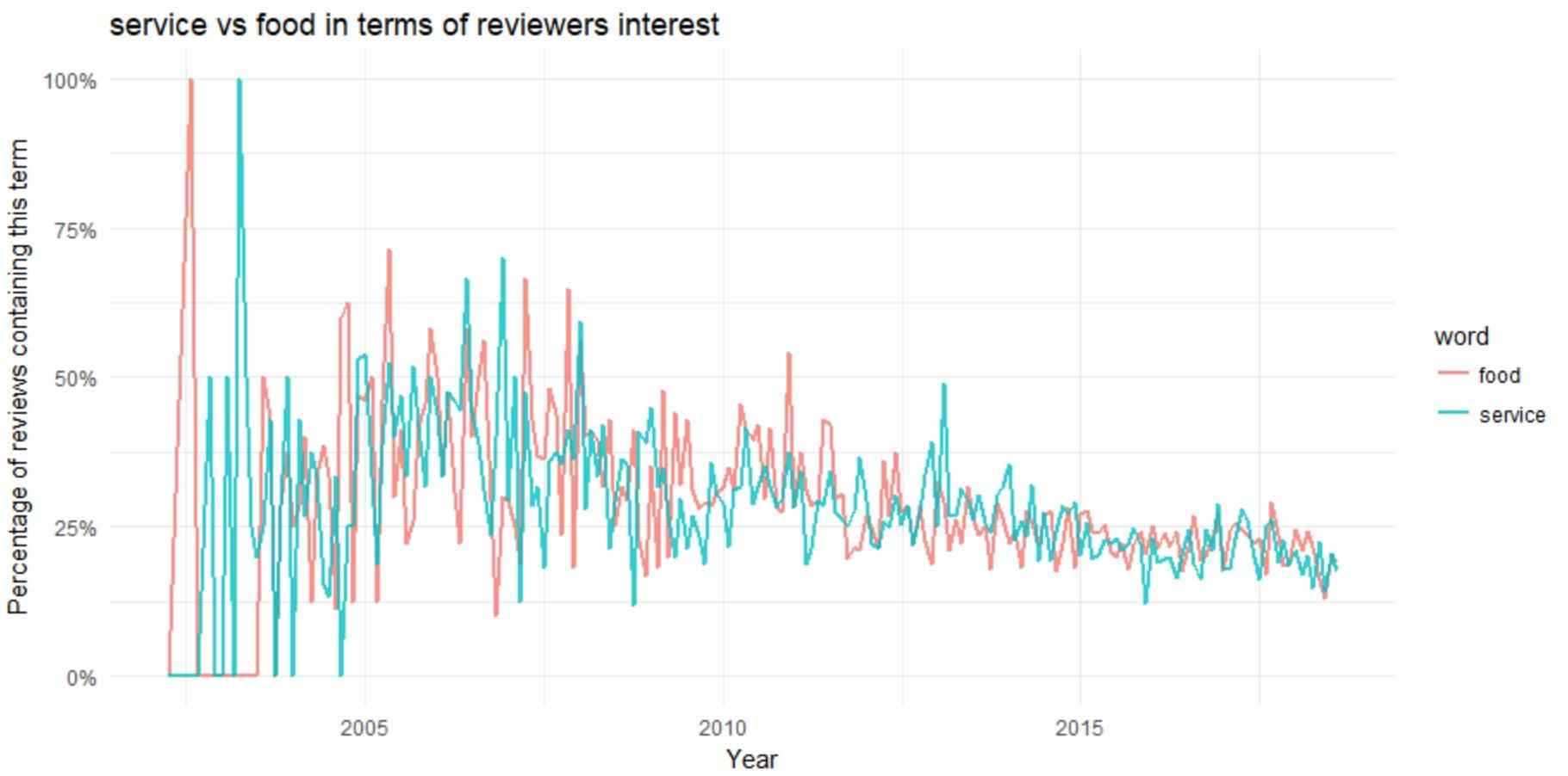
Service and food both were trending topics before 2010. The discussion regarding food and service topics peaked at starting of the data around 2003, then it was a downward trend after 2005.
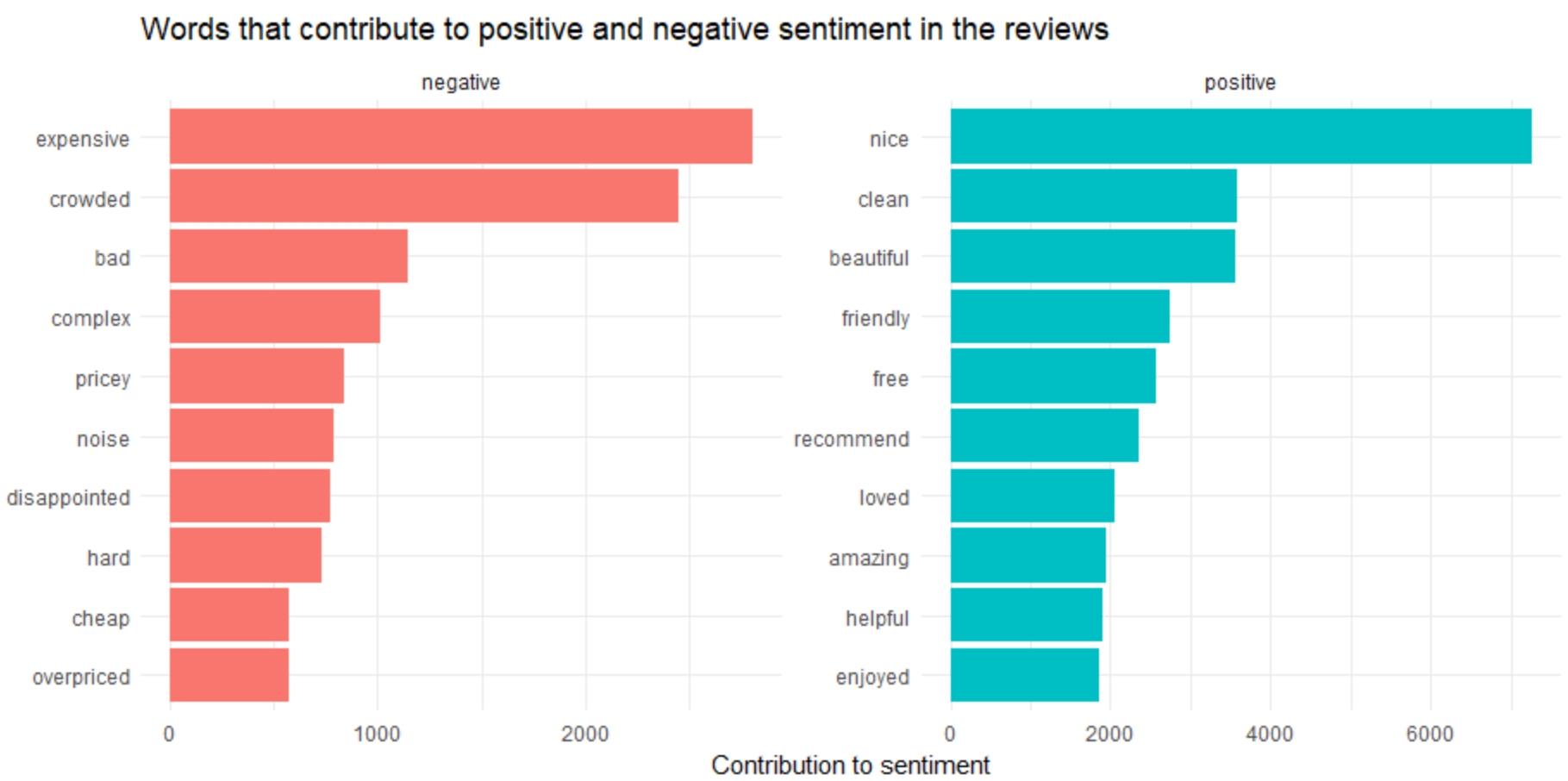
We aim to regulate the attitude of a reviewer, concerning his or her past involvement or emotional reaction towards the hotel. The attitude may be a sentence or valuation.
The common positive and negative words in the comments are fetched by below given Python script:
reviews <- df %>%
filter(!is.na(review_body)) %>%
select(ID, review_body) %>%
group_by(row_number()) %>%
ungroup()
tidy_reviews <- reviews %>%
unnest_tokens(word, review_body)
tidy_reviews <- tidy_reviews %>%
anti_join(stop_words)

bing_word_counts <- tidy_reviews %>%
inner_join(get_sentiments("bing")) %>%
count(word, sentiment, sort = TRUE) %>%
ungroup()

bing_word_counts %>%
group_by(sentiment) %>%
top_n(10) %>%
ungroup() %>%
mutate(word = reorder(word, n)) %>%
ggplot(aes(word, n, fill = sentiment)) +
geom_col(show.legend = FALSE) +
facet_wrap(~sentiment, scales = "free") +
labs(y = "Contribution to sentiment", x = NULL) +
coord_flip() +
ggtitle('Words that contribute to positive and negative sentiment in the reviews')
Let us try another script to check whether the results are same or not.
contributions <- tidy_reviews %>%
inner_join(get_sentiments("afinn"), by = "word") %>%
group_by(word) %>%
summarize(occurences = n(),
contribution = sum(score))
contributions %>%
top_n(25, abs(contribution)) %>%
mutate(word = reorder(word, contribution)) %>%
ggplot(aes(word, contribution, fill = contribution > 0)) +
ggtitle('Words with the greatest contributions to positive/negative
sentiment in reviews') +
geom_col(show.legend = FALSE) +
coord_flip()
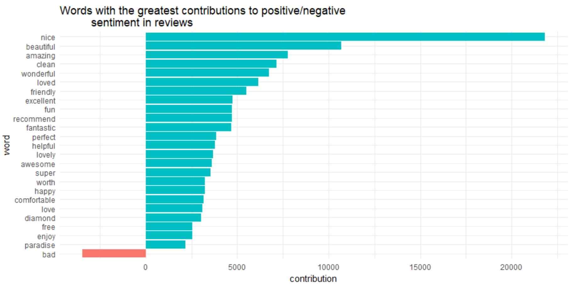
“diamond” is marked as positive sentiment in the graph.
Using Bigrams to Insert Context in Sentiment Analysis
Let us check how frequently words are preceded by “not” word
not_words %>%
mutate(contribution = n * score) %>%
arrange(desc(abs(contribution))) %>%
head(20) %>%
mutate(word2 = reorder(word2, contribution)) %>%
ggplot(aes(word2, n * score, fill = n * score > 0)) +
geom_col(show.legend = FALSE) +
xlab("Words preceded by \"not\"") +
ylab("Sentiment score * number of occurrences") +
ggtitle('The 20 words preceded by "not" that had the greatest contribution to
sentiment scores, positive or negative direction') +
coord_flip()
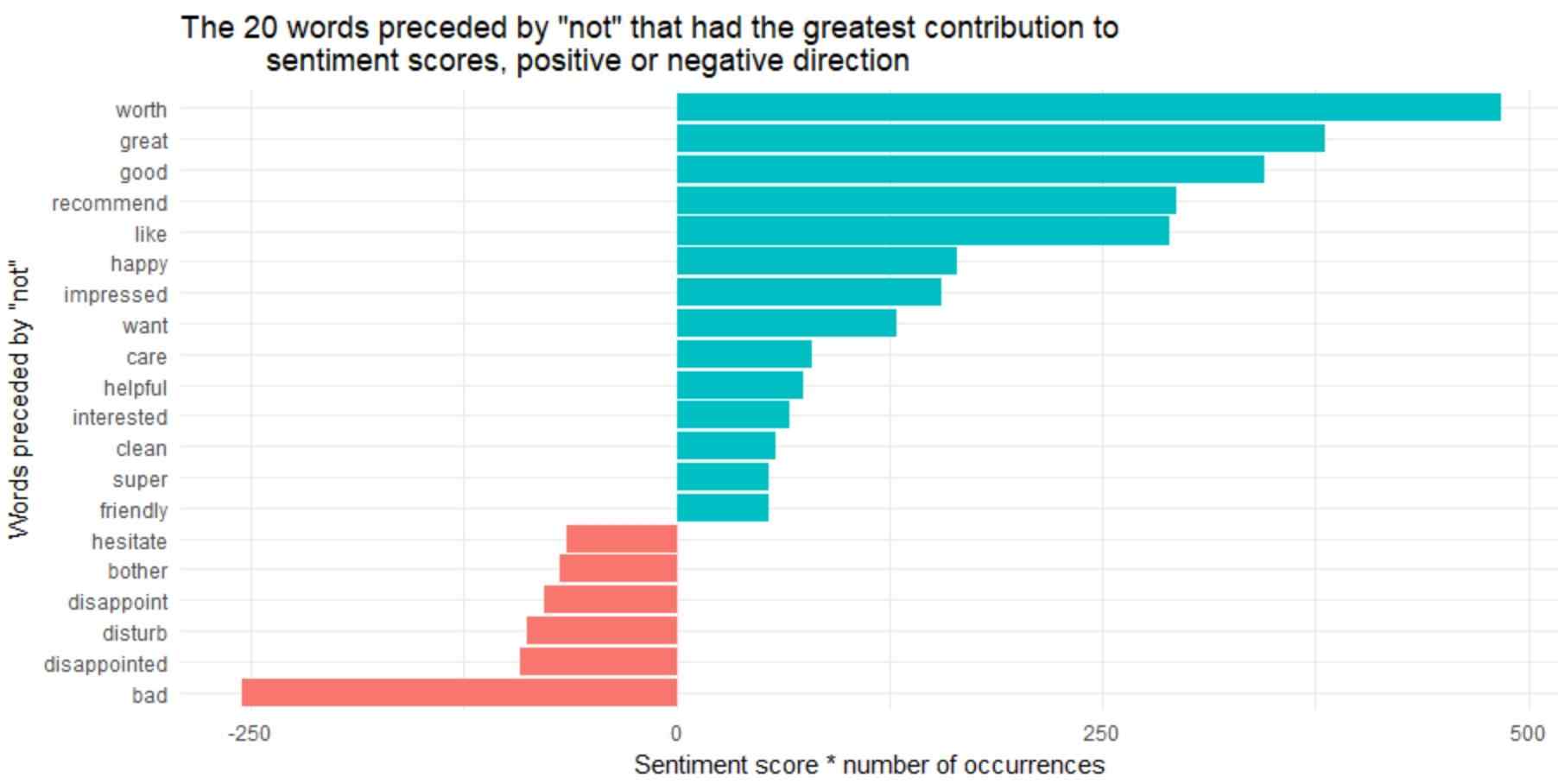
The bigrams “not worth”, “not great”, “not good”, “not recommended” and “not like” were the reasons behind the cause of miss-identification, making the text seem more positive than always.
Except “not”, there are few words that negate the subsequent term, for example ‘no”, “never”, and “without”. Let us check the script
negation_words <- c("not", "no", "never", "without")
negated_words <- bigrams_separated %>%
filter(word1 %in% negation_words) %>%
inner_join(AFINN, by = c(word2 = "word")) %>%
count(word1, word2, score, sort = TRUE) %>%
ungroup()
negated_words %>%
mutate(contribution = n * score,
word2 = reorder(paste(word2, word1, sep = "__"), contribution)) %>%
group_by(word1) %>%
top_n(12, abs(contribution)) %>%
ggplot(aes(word2, contribution, fill = n * score > 0)) +
geom_col(show.legend = FALSE) +
facet_wrap(~ word1, scales = "free") +
scale_x_discrete(labels = function(x) gsub("__.+$", "", x)) +
xlab("Words preceded by negation term") +
ylab("Sentiment score * # of occurrences") +
ggtitle('The most common positive or negative words to follow negations
such as "no", "not", "never" and "without"') +
coord_flip()
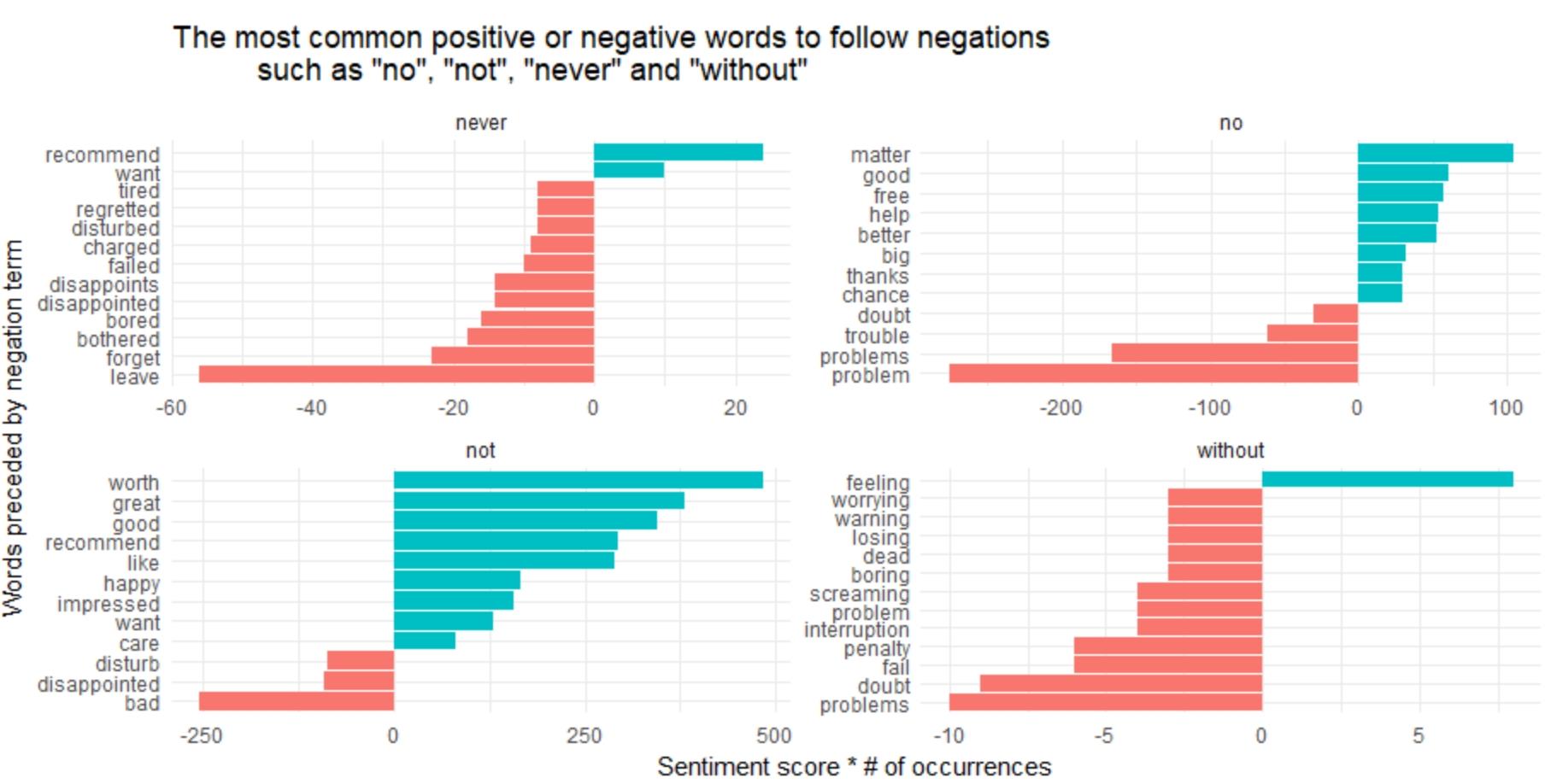
It seems to be the greatest source of misidentifying a word as positive comes from “not worth/great/good/recommend”, and the biggest source of incorrectly distinguished sentiments is “not bad” and “no problem”.
Now, let us write the Python script for web scraping of positive and negative reviews.
sentiment_messages <- tidy_reviews %>%
  inner_join(get_sentiments("afinn"), by = "word") %>%
  group_by(ID) %>%
  summarize(sentiment = mean(score),
            words = n()) %>%
  ungroup() %>%
  filter(words >= 5)sentiment_messages %>%
  arrange(desc(sentiment))
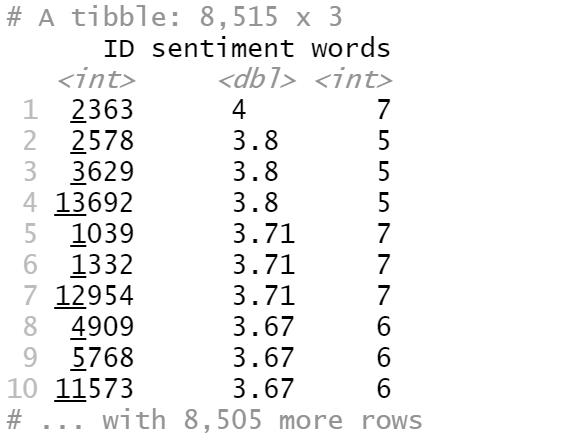
From the above image, we can find that the most positive review’s ID is 2363
f[ which(df$ID==2363), ]$review_body[1]
For negative comments, the Python script is mentioned as:
df[ which(df$ID==3748), ]$review_body[1]]
The most negative review’s ID is: 3748
For any further queries, contact us!!
 ✯ Alpesh Khunt ✯